Cancel
Data
Insight
Strategy
Communities
Solutions
Commodities
About Us
Press & Media
Careers
CRU Online
Get in Touch
Home
Communities
Thought Leadership
Thought Leadership
Filter By
Clear Filters
Location
Show
Africa
Show
North Africa
Show
Egypt
Southern Africa
Americas
Show
Central America
Show
Mexico
North America
Show
Canada
United States of America
South America
Show
Argentina
Brazil
Chile
Asia
Show
East Asia
Show
China
Republic of Korea (South)
South Asia
Show
India
Southeast Asia
Show
Indonesia
Thailand
Europe
Show
Eastern Europe
Show
Russia
Southern Europe
Show
Italy
Western Europe
Show
Germany
Middle East
Oceania
Show
Australia
Commodities
Show
Aluminium
Show
Aluminium
Aluminium Products
Show
Beverage Can Sheet
Rolled Products
Bauxite & Alumina
Show
Alumina
Bauxite
Carbon Products
Show
Anodes
Calcined Pet Coke
Coal Tar Pitch
Recycled Aluminium
Base Metals
Show
Chrome
Copper
Show
Copper Concentrates
Copper Scrap
Lead
Show
Lead Concentrates
Molybdenum
Nickel
Tin
Zinc
Show
Zinc Concentrates
Battery Materials
Show
Battery Raw Materials
Show
Lithium
Cobalt
Battery-grade manganese
Battery-grade phosphates
Battery Active Materials
Battery Cells
Battery Recycling
Energy Commodities
Show
Gas
Hydro power (Water)
Hydrogen
Oil
Solar
Thermal Coal
Uranium
Wind
Electricity
Ferroalloys
Show
Electrolytic Manganese
Ferrochrome
Ferromanganese
Ferrosilicon
Ferrovanadium
Manganese Ore
Silicomanganese
Silicon Metal
Fertilizers
Show
Ammonia
Nitrates and Sulphates
Show
AN
Nitrogen
Phosphates
Show
DAP/MAP
NP/NPKs
Phosphate Rock
Potash
Show
MOP
SOP
Sulphur
Sulphuric Acid
Urea
Water Soluble
Minor Metals
Show
Rare Earth Metals
Tungsten
Vanadium
Precious Metals
Show
Gold
PGMs
Silver
Steel
Show
Flat Products
Show
Steel Plate
Steel Sheet
Hot Rolled Coil (HRC)
Long Products
Stainless Steel
Steelmaking Raw Materials
Show
Iron Ore
Metallurgical Coal
Metallurgical Coke
DRI/HBI & Pig Iron
Electrical Steels
Scrap
Wire & Cable
Show
Communication Cable
Show
Fibre Optic Subsea
Optical Fibre & Cable
Energy Cable
Show
HV & EHV Cable
Silicon
Topics
Show
Prices
Show
Price Assessment
Green Premia
Price Forecast
Battery
Show
Battery Raw Materials
Economics
Show
Budget
Supply
Demand
Import/Export
Exchange Rates
Inflation
Interest Rates
Household
Production
Trade
Show
Section 232
Tariffs & Quotas
Trade War
Show
Trade Developments
Strategy
Show
Corporate
Show
Capex
M&A
Financing
Investment Opportunities
Wire & Cable
Show
Communication cable
Energy cable
Fertilizers & Agricultural Chemicals
Chemicals
Show
Petrochemical producer
Transport
Show
Automotive
Freight
Shipping
Construction
Show
Infrastructure
Metals
Mining
Show
Mining & Extraction
Smelting & Refining
Manufacturing
Technology
Show
Electronics
Green Technology
Government and Institutions
Show
Policy/Regulation
Defence
Financial Services
Show
Traders
Investors
Energy & Renewables
Show
Energy Transition
Show
Energy Storage
Utilities
Show
Power Generation
Electricity
Power Transmission
Emissions
Show
Green Commodities
Decarbonisation
Show
Green Technology
Carbon markets
Carbon trading
GHG Emissions
Show
Carbon Emissions
Scope 1
Scope 2
Scope 3
Climate Risk
Climate Change
Industries
Show
Batteries
Power, Energy, Renewables and Utilities
Wire and Cable (& Fibre)
Fertilizers
Transport & Automotive
Mining, and Metal Production
Manufacturing & Fabrication
Stockholders/Distributors
Government and Policymakers
Financial Services, Investors and Traders
Showing 1-12
Results of 969
Increased demand for metals for defence poses procurement risk
3rd July 2025
Western vanadium producers are on the rocks as prices disappoint
2nd July 2025
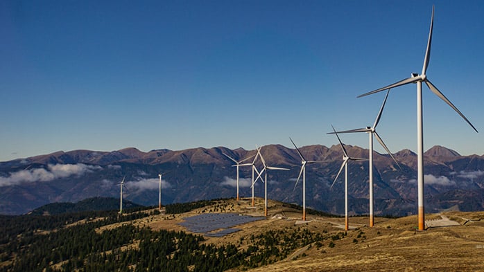
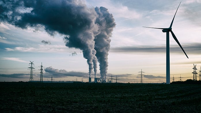
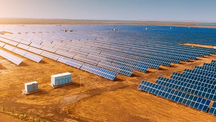
Strong wind power will lower carbon price, but economic uncertainty persists
27th June 2025
CRU aluminium conference: Trade, tariffs and recycling takeaways
24th June 2025
Israel-Iran war poses major risks for energy markets
17th June 2025
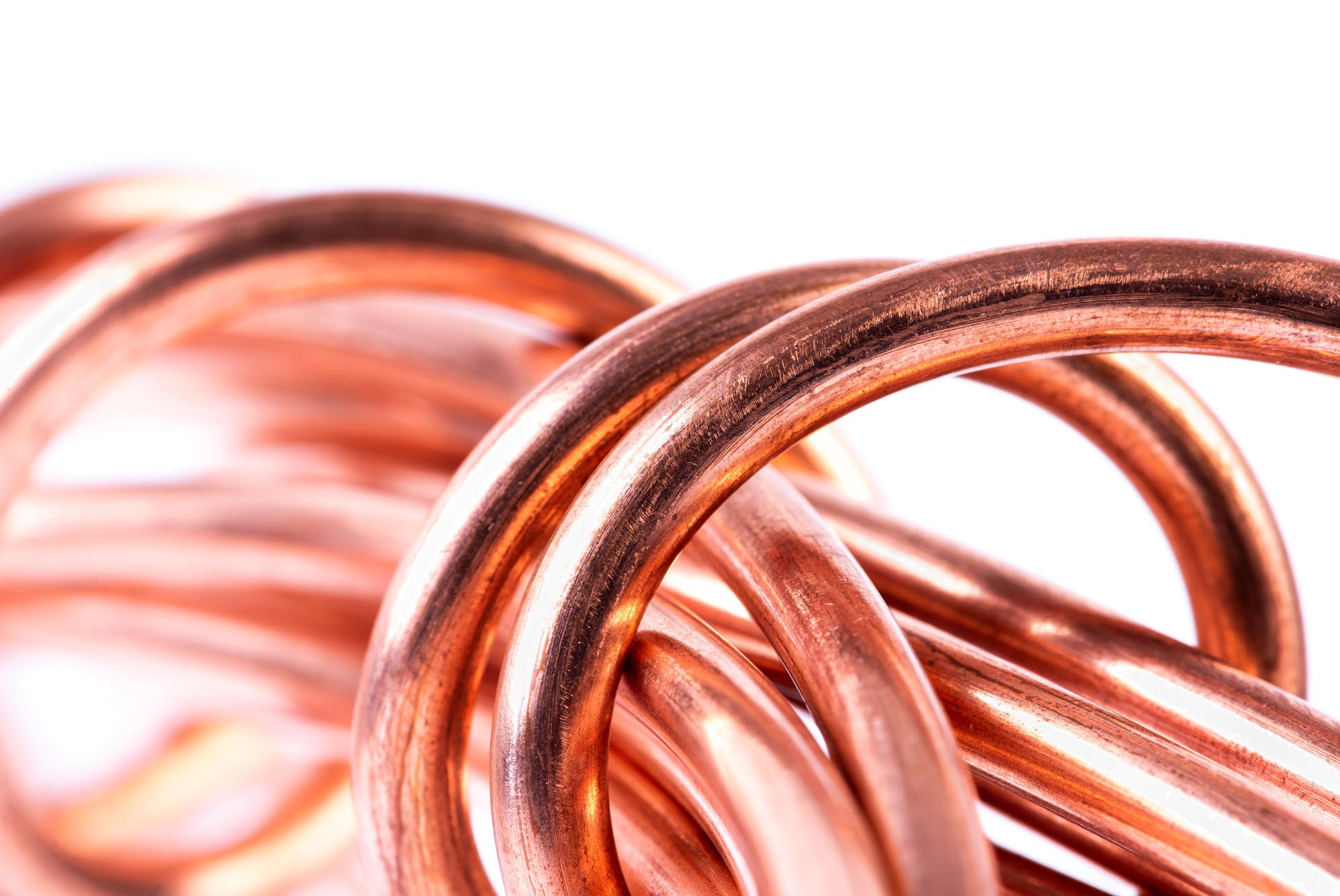
BHP’s copper conundrum: To buy or to build
16th June 2025
2025/2026 China Mobile optical cable tender awards released
11th June 2025
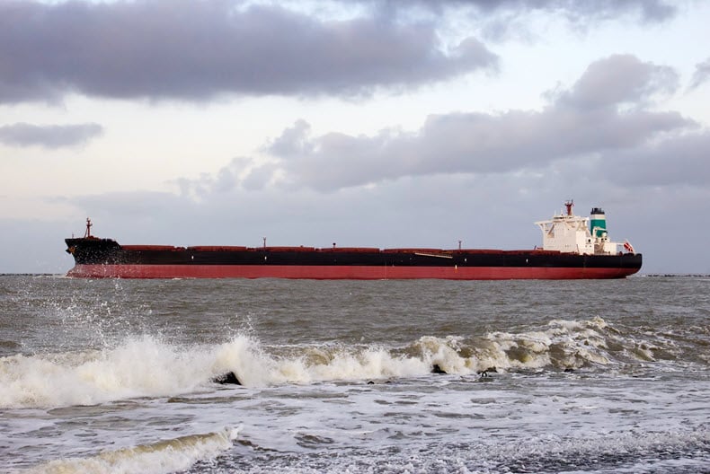
FiberConnect 2025: Industry resilience meets fibre policy uncertainties
10th June 2025
Continued economic weakness and strong winds will lower the EU carbon price in June
2nd June 2025
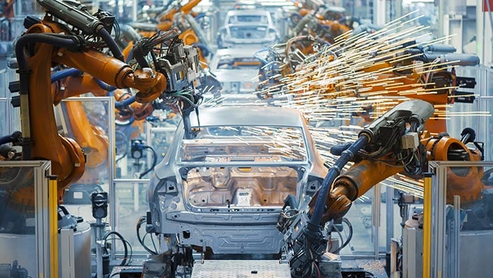
Automakers regionalise to mitigate risk and boost sales
27th May 2025
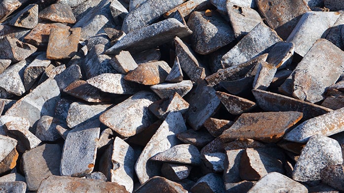
Direct reduced iron to become one of the fastest growing commodities within the steel value-chain
27th May 2025
How has HPQ demand and supply emerged as a hot topic?
14th May 2025
Load More